Trends in Space
In this page we will explore where UFO sightings are reported in the United States. First we will visualize where throughout the U.S. these reports are being made, and then compare reports made in urban/suburban areas (i.e. close to major cities), and those made in rural areas (i.e. far from major cities). We separate these two groups using a cutoff criteria of being within 5 miles of a city with more than 200,000 residents.
## Default packages & settings
# Load packages
library(tidyverse)
library(knitr)
library(leaflet)
library(usmap)

# Set seed for reproducibility
set.seed(1)

# Set default figure options
knitr::opts_chunk$set(
  fig.width = 6,
  out.width = "90%"
)

theme_set(theme_bw() + theme(legend.position = "bottom"))

options(
  ggplot2.continuous.colour = "viridis",
  ggplot2.continuous.fill = "viridis"
)

scale_colour_discrete = scale_colour_viridis_d
scale_fill_discrete = scale_fill_viridis_d

## Data import
# Import UFO data
df_ufo = read_csv("data/ufo_clean.csv")

# Add population data
df_pop =
  read_csv("data/us_census.csv") |>
  rename(state = abbrv) |>
  select(state, census_2010)
Reports across the U.S.
Raw Data
To begin, we simply visualize a random 2% of these reports to get a sense of where these sightings are throughout the country.
df_ufo |>
  sample_frac(0.02) |>
  leaflet() |>
  addProviderTiles(providers$CartoDB.Positron) |>
  addCircleMarkers(~city_longitude,~city_latitude, radius = 1)
At first glance, these reports seem to cluster along the coasts and in other regions of high population density. So, we will adjust for population at the state level and re-visualize the results.
Population-adjusted reports
df_ufo |>
  group_by(state) |>
  summarize(n_obs = n()) |>
  left_join(df_pop, by = join_by(state)) |>
  mutate(obs_per = n_obs/census_2010*100000) |>
  plot_usmap(data = _, values = "obs_per", color = "#333333") +
  labs(
    title = "UFO Reports per 100,000 Population"
  ) +
  scale_fill_continuous(name = "Reports per 100k") +
theme(legend.position = "bottom") 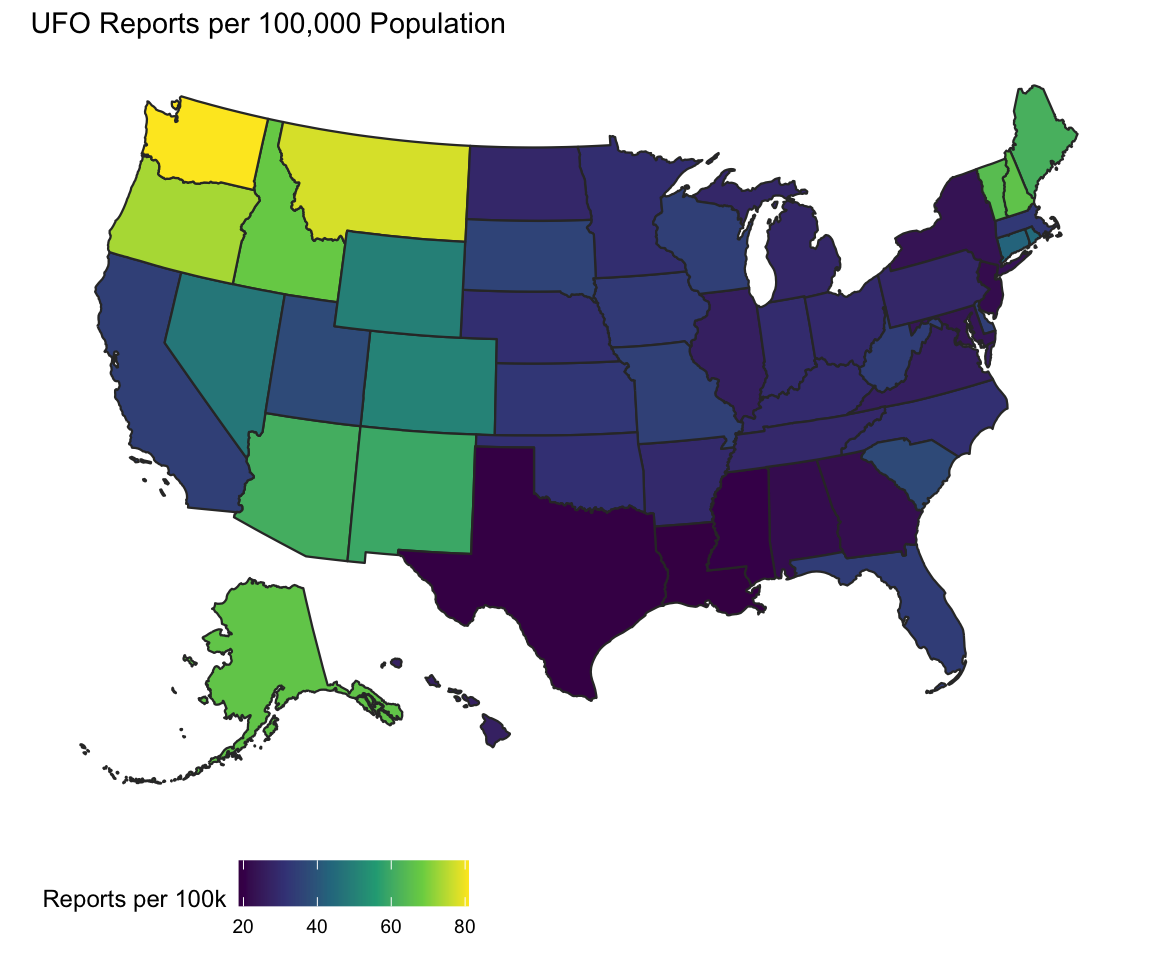
This heatmap reveals three clusters with particularly high UFO reports. The Northwest, including Washington, Oregon, Idaho, Montana, and Alaska are the 5 states with the highest population-adjusted UFO reports ranging from 66 (AK) to 81 (WA) UFO reports per 100,000 residents. Next is northern New England, with New Hampshire, Vermont, and Maine taking positions 6-8 in the list. These states have between 61 (ME) and 66 (NH) UFO reports per 100,000. Rounding out the top 10, we have Arizona and New Mexico, with 61 and 59 reports per 100,000 residents, respectively.
Table 1. States with highest reports per 100,000 population
## Table form
df_ufo |>
  group_by(state) |>
  summarize(n_obs = n()) |>
  left_join(df_pop, by = join_by(state)) |>
  mutate(obs_per = n_obs/census_2010*100000) |>
  arrange(desc(obs_per)) |>
  head(10) |>
  kable(
    col.names = c("State", "Number of UFO Sightings",
                  "Population (2010 census)", "UFO sightings per 100k"),
digits = 1)| State | Number of UFO Sightings | Population (2010 census) | UFO sightings per 100k |
|---|---|---|---|
| WA | 5443 | 6724540 | 80.9 |
| MT | 768 | 989415 | 77.6 |
| OR | 2818 | 3831074 | 73.6 |
| ID | 1062 | 1567582 | 67.7 |
| AK | 473 | 710231 | 66.6 |
| NH | 871 | 1316470 | 66.2 |
| VT | 405 | 625741 | 64.7 |
| ME | 818 | 1328361 | 61.6 |
| AZ | 3894 | 6392017 | 60.9 |
| NM | 1223 | 2059179 | 59.4 |
If we cluster the number of observations by nearest large city, we see a similar result. The two cities with the most UFO sightings nearby are are Seattle, WA and Portland, OR. These are large cities but not the largest in the U.S. The West Coast seems to have more reports than other areas, though St. Louis is a bit of an outlier in this regard.
Table 2. Cities with most sightings nearby
df_ufo |>
  group_by(closest_city) |>
  summarize(n_obs = n()) |>
  arrange(desc(n_obs)) |>
  head(10) |>
kable()| closest_city | n_obs |
|---|---|
| Portland | 2646 |
| Seattle | 2472 |
| Chicago | 1842 |
| Los Angeles | 1378 |
| St. Louis | 1361 |
| Atlanta | 1332 |
| Sacramento | 1254 |
| Arlington | 1211 |
| Philadelphia | 1191 |
| Spokane | 1174 |
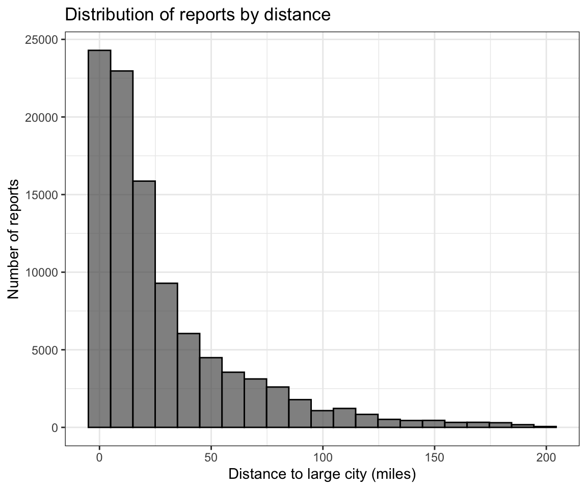
Distance to cities
We also plotted the distribution of the dist variable,
the distance to the nearest city of at least 200,000 residents. This
histogram shows that the most reports occur close to large cities, but
there is a long tail of reports that were made further away. There are
also 1065 reports that were made further than 200 miles from a large
city, and 90 that were more than 400 miles away.
df_ufo |>
  filter(dist <= 200) |>
  ggplot(aes(x = dist)) +
  geom_histogram(bins = 21, alpha = 0.7, col = I("black")) +
  labs(
    title = "Distribution of reports by distance",
    y = "Number of reports",
    x = "Distance to large city (miles)"
) 
Rural vs Urban Differences
With this preliminary understanding of the geographic distribution of
UFO reports, we wanted to explore if the distance from large cities is
related to characteristics of the report. To do this, we separate
reports into urban/suburban and rural
categories, using a cutoff value of 5 miles to a large city. This is not
a perfect division, as this distinction should really be done by
population density, but should be servicable to identify major
differences, as will be seen below.
UFO Shape
Our first question was whether the type of object reported differed between these group, as determined by the shape of the UFO.
df_loc_shape =
  df_ufo |>
  group_by(location, shape) |>
  summarize(n_obs = n()) |>
  arrange(desc(n_obs)) |>
  pivot_wider(
    names_from = "location",
    values_from = "n_obs"
  )

df_loc_shape |>
  head(10) |>
kable(col.names = c("Shape", "Rural", "Urban/Suburban"))| Shape | Rural | Urban/Suburban |
|---|---|---|
| light | 16728 | 5065 |
| circle | 8559 | 2632 |
| triangle | 7531 | 2210 |
| fireball | 5714 | 1864 |
| unknown | 5482 | 1648 |
| other | 5298 | 1749 |
| sphere | 5130 | 1722 |
| disk | 4098 | 1381 |
| oval | 3360 | 1116 |
| formation | 2677 | 848 |
Both rural and urban reports look similar, with the same ranking of
the reported shapes. The most common descriptor of the UFO was just a
light, followed by either circle or
triangle. To analyze whether descriptions of UFOs varied
between these groups, we conducted a Chi-Squared test of homogeneity.
This revealed that the distribution of shapes did differ significantly
between the urban/suburban and rural categories.
df_loc_shape |>
  select(-shape) |>
  as.matrix() |>
  chisq.test()
##
## Pearson's Chi-squared test
##
## data: as.matrix(select(df_loc_shape, -shape))
## X-squared = 72.097, df = 22, p-value = 3.082e-07This result is not being influenced by the comparatively few observations for some shapes. If the data set is restricted to only the top 10 or top 15 shapes, the p-value is still far below 0.05.
Encounter Duration
Next, we wish to consider whether the length of UFO encounters is different between the urban/suburban and rural groups. First, we will look at the data, which skewed right (more observations on the second scale than the minute scale, and more on the minute scale than the hour scale). So to understand the distribution, we will look at the data on the log scale.
df_ufo |>
  drop_na(duration_clean) |>
  filter(duration_clean != 0) |>
  ggplot(aes(x = duration_clean, fill = location)) +
  geom_histogram(alpha = 0.5, bins = 41, col = I("black")) +
  scale_x_continuous(
    trans = "log10",
    breaks = scales::trans_breaks("log10", function(x) 10^x),
    labels = scales::trans_format("log10", scales::math_format(10^.x))
                     ) +
  labs(
    title = "Distribution of encounter duration",
    y = "Number of reports",
    x = "Encounter Duration (seconds)",
    fill = "Location"
  )
Even though the data are highly right-skewed, there are enough observations that it is still valid to compare the data using a t-test. There are 1266 reports with a duration over 2 hours, comprising about 1% of the sample. These reports range from several hours to several months. I will restrict the comparison of the data to those with encounters lasting at most hours.
df_ufo |>
  drop_na(duration_clean) |>
  filter(duration_clean <= 7200) |>
  t.test(duration_clean ~ location, data = _)
##
## Welch Two Sample t-test
##
## data: duration_clean by location
## t = 6.2378, df = 38429, p-value = 4.485e-10
## alternative hypothesis: true difference in means between group rural and group urban is not equal to 0
## 95 percent confidence interval:
## 38.34605 73.48570
## sample estimates:
## mean in group rural mean in group urban
## 625.4033 569.4874The results of this test suggest that there is a significant difference between the average duration of the rural UFO sightings and the urban UFO sightings. We estimate that sightings in rural areas last for approximately one minute longer than sightings in urban areas (10.5 minutes vs. 9.5 minutes).